Raptor - A High Level Algorithmic Skeleton CUDA Library
Apr 7, 2024 | Github: github.com/dma-neves/raptor
Index
- 1. Introduction
- 2. Basics
- 3. Skeletons
- 4. Collections
- 5. Targets
- 6. Raptor Function
- 7. Raptor vs Thrust
- 8. Performance
- 9. Conclusions
1. Introduction
CUDA is a great tool for accelerating massively paralelizable applications on the GPU. However, its utilization can be complex and verbose. Writing programs in plain CUDA involves: management of host and device memory, kernel execution and synchronization, grid and block size definition, etc. Some higher level libraries, such as thrust, have already simplified and abstracted a lot of these concepts, allowing the programmer to focus on the problem related logic, instead of constantly having to deal with all of the GPU intricacies. Even so, we believe we can go further. Raptor is a high level algorithmic skeleton CUDA library which allows the user to define all their parallel computations using a set of smart containers, algorithmic skeletons, and raptor functions, while achieving very similar performance as programs written in thrust.
Raptor's syntax and core design features are taken from marrow.
Similarly to marrow, raptor provides a set of smart containers (vector, array, vector<array>, scalar) and skeletons
(map, reduce, scan, filter, sort) that can be applied over the smart containers. Containers can store the
data both on the
host (CPU) and device (GPU), and expose a seemingly unified memory address space. Skeletons are executed on the device. Any necessary containers are
automatically and lazily allocated and uploaded whenever a skeleton is executed. Similarly to marrow,
raptor also provides a generic function primitive. A raptor function allows one to specify a generic device function that can operate over
multiple raptor containers of different sizes & types, basic data types, and GPU coordinates.
Before proceeding, note that this guide assumes a basic knowledge of C++ (including functors and basic templates), CUDA, and common high-order functions such as map, filter, reduce, scan.
2. Basics
Lets start with one of the most basic parallel programs, saxpy. saxpy is a function that takes as input two vectors of equal size x and y, and
a single scalar a, and outputs a*x + y, i.e the output is a vector res, such that res[i] = x[i]*a + y[i],
for all indices i from 0 to the size of the vectors.
struct saxpy {
    __device__
    float operator()(float x, float y, float a) {
        return a*x + y;
    }
};

int main() {

	int n = 1e6;
    float a = 2.f;
    vector<float> x(n);
    vector<float> y(n);
    x.fill(4.f);
    y.fill(3.f);

    vector<float> res = map<saxpy>(x,y,a);
}
As we can see, compared to a CUDA implementation, raptor abstracts all host-device communication and setup. The programmer simply defines a set of containers and applies skeletons over them. Raptor then parallelizes these computations on the GPU.
We start by defining a device functor saxpy that describes the computation of a single element of the result. In the main
function, we start by initialing our inputs using a similar syntax to the standard C++ library. Note that this code assumes we are using the raptor namespace,
otherwise, we would instantiate a raptor vector as raptor::vector. In the last line of main, we apply the map skeleton
to the three inputs, using the saxpy functor as the mapping function, and store the result in the res vector.
In the background,
x and y are initially allocated and filled on the host (we could also decide to fill them directly on the device - more on this later),
then, when the map skeleton is invoked, the vectors are uploaded to the device, and raptor launches a CUDA kernel that applies the saxpy
functor to all the elements of x and y. Additionally, raptor also allocates the result vector automatically. Its worth noting
that even though the saxpy functor takes three floats as input, we pass to the map skeleton two vectors of floats, and an additional single float.
At compile time, raptor resolves all of the skeleton and function arguments. Raptor containers are distributed to the kernel threads (one element per thread),
and basic data types (like the argument a) are passed directly.
We now present a slightly more complex program that takes advantage of multiple skeletons: the discrete riemann sum.
This program computes a discrete area under a function, i.e an approximation of a function's integral. We define
the integrating function in the device function fun. The body of fun can be replaced with any desired function.
__device__
static float fun(float x) {
    return pow(x, 4.f) * (-5.56) + pow(x, 3.f) * 1.34 + x * x *  3.45 + x * 5 + 40;
}

struct compute_area {
    __device__
    float operator() (float index, int start, float dx) {
        float x = (float)start + index*dx;
        float y = fun(x);
        return dx * y;
    }
};


float riemann_sum(int start, int end, int samples) {

    float dx = (float)(end - start) / (float)(samples);
    vector<float> indexes = iota<float>(samples);
    vector<float> vals = map<compute_area>(indexes,start, dx);
    scalar<float> result = reduce<sum<float>>(vals);
    return result.get();
}
Once again, we start by defining a device functor compute_area, which describes the computation of a single element of the result.
We compute the y value for the corresponding x and multiply it by the discrete Δriemann_sum function,
we start by creating a vector of counting indices using the iota function. This function is provided by raptor and generates a vector of
size N with the values {0,1,2,...,N}. We then apply the map skeleton to the indices
(and also pass the necessary start and dx arguments), using the compute_area functor as the mapping
function, and store the result in the vals vector. This vector will contain the N discrete areas we want to sum.
Finally, we sum all the values with the reduce skeleton, using the sum operator (provided by raptor) as the reducing function,
and store the result in a scalar. Scalars single element containers that can store a value both on the host and device. We
can use the get function to obtain the stored value.
3. Skeletons
The current supported skeletons are:
map: This skeleton can receive any number of raptor containers of any type (but should have same size), and any number of basic data types. The main type restriction is tied to the first parameter which must be a collection (vector,arrayorvector<array>) dictating the return type. Additionally,mapreceives as a template parameter a device functor describing the mapping function. The skeleton returns the container with the mapped values.filter: This skeleton must receive either a collection and a filtering functor, or two collections of equal size. The first being the collection to filter, and the second a collection of integers containing0s and1s. A value of0excludes the corresponding element, while a value of1includes the corresponding element. The skeleton returns a container with the filtered set of elements.reduce: This skeleton must receive a single collection, and receive as a template parameter a device functor describing the reducing function. The skeleton returns a single reduced value.scan: This skeleton must receive a single collection, and receive as a template parameter a device functor describing the scanning function. The skeleton returns a container of equal size containing the scanned values.sort: This skeleton must receive a single collection of comparable types, and returns a container with all the elements sorted in ascending order.
Besides these skeletons, raptor also provides a set of common operators which can be used alongside the map, reduce, and scan skeletons.
These operators include: sum, sub, mult, max and min.
4. Collections
4.1. Vector & Arrays
Both rator::vector and raptor::array follow a similar syntax to the std::vector and std::array respectively.
This means these collections include basic functions such as size, fill, [], push_back, etc.
The main difference, from a user perspective, lies in the get and set functions. In order to read a value from a collection, we can use the get
function. Updating an element can be performed using the set function. The set function marks the collection (or element) as dirty, meaning
that if a skeleton is later applied over said collection, it will be properly synchronized to the device. Collections also support the subscript operator [].
The subscript operator is similar to the get function but marks the container (or element) as dirty. This means that writes: col.set(i, val)
can alternatively be expressed as: col[i] = val.
Internally, raptor stores two versions of a collection, a host version, and a device version. Typically, updates are performed on the host and later synchronized to the device.
However, sometimes containers are never accesses on the host or vice versa. Raptor adopts an optimization such that memory is only allocated whenever it is accessed or
manipulated. This means, that a container can be either allocated only on the host, only on the device, on both, or not allocated at all. For example, in the previous saxpy example,
we instantiate the vector x using: vector<float> x(n). This vector is initially not allocated. When we fill (host fill) it with the value 4.f,
the vector is automatically allocated on the host. We then apply the map skeleton over it:
map<saxpy>(x,y,a). This results in the container being automatically allocated on the device. Since the vector was already allocated and dirtied on
the host, the contents of the the host vector is also transferred to the device after allocation.
It is important to note that raptor containers only store pointers (smart pointers) to the actual data. This means that the containers are extremely light
objects that can easily be copied. All copies are therefore shallow. In order to perform a deep copy, we must use the provided copy function:
a.copy(b).
When we instantiate a raptor collection, we can optionally set its synchronization granularity by passing a sync_granularity enum value to
the constructor. The default granularity is coarse grain. A coarse grain granularity implies that whenever a collection has been manipulated on the host
and must be uploaded to the device, the entire collection is uploaded. For example, if we change the first element of a large vector that is already allocated
on the host and device, and then apply a skeleton over it, the entire vector is uploaded. On the other hand, a fine granularity implies that whenever a collection has been
manipulated on the host and must be uploaded to the device, only the dirty elements are uploaded. Returning to the previous example, only the first
element would be uploaded as the rest would remain unchanged. This might be useful when dealing with vectors that store heavy objects and are subjected
to sporadic updates.
4.2. Vector of Arrays
GPUs work best when dealing with contiguous data, however, some problems require dynamic data structures that can efficiently mutate. Such data structures can often
be implemented using multiple fixed size contiguous blocks. For example, a linked list is usually not well suited for a GPU environment, a blocked adjacency list on the
other hand, can offer both good memory locality (depending on the size of the blocks) and efficient mutability. For this reason, raptor offers the vector<array<N,T>>
collection. This collection allows us to define a vector of fixed size arrays that can efficiently grow, shrink, and be updated.
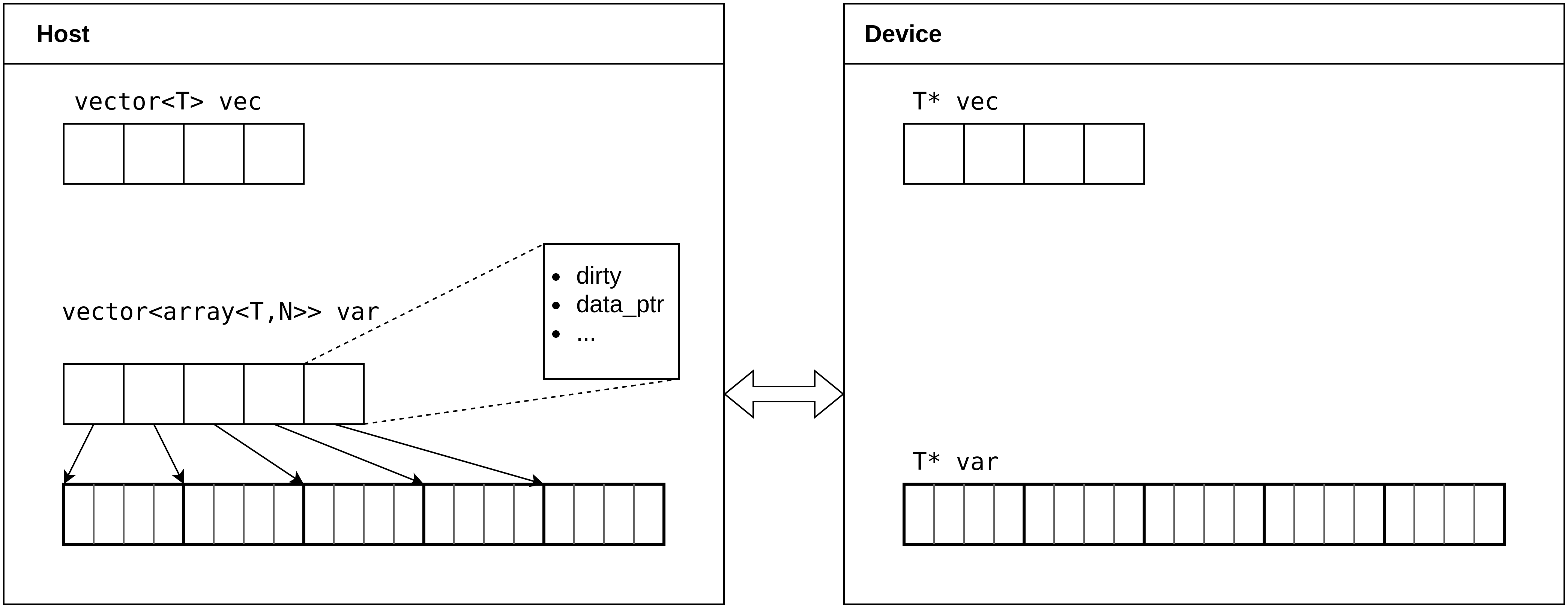
Figure 1 displays the memory layout of a vector and a vector of arrays that have been allocated both on the host and device.
As we can see, a normal collection, such as vec, is simply stored as a contiguous array on the
host, and has a replica stored on the device. The vector<array<N,T>> has a more nuanced storage layout.
Assuming a fixed array size of N and a variable vector size of
S, a vector<array<N,T>> is stored on the host using two data structures. A contiguous block of data of length N*S, and a vector
of arrays of length S. These arrays only contain metadata, and point
to the contiguous memory block. This allows for user-friendly manipulations of the data structure on the host, while allowing for
efficient memory transfers and memory accesses on the device. If
the host would only store a vector of arrays containing the actual data,
transferring the whole vector to the device would require N separate memory transfers, rather than a single large memory transfer
of N*S*sizeof(T) bytes. Furthermore, by storing a vector of arrays on the host, we gain the ability to track individual dirty arrays.
When synchronizing the vector of arrays to the device, assuming it has already been allocated, only the dirty arrays need to be
synchronized, rather than the entire vector. This data structure is defined to use a fine synchronization granularity by default.
This targeted synchronization approach enhances efficiency by minimizing unnecessary
data transfers.
5. Targets
Both the copy and fill functions are resource-intensive tasks. For this reason, raptor performs most of these tasks
asynchronously (the exceptions are host fill with values different than 0 and host fills using functors).
If another operation is applied to a container still undergoing an asynchronous task, synchronization is automatically ensured. Moreover,
raptor offers users the flexibility to specify the target of these tasks as either the host or the device. The default target is the host, but
it can be overridden via a template parameter. Returning to our saxpy example, we could fill x and y
directly on the device using:
x.fill<DEVICE>(4.f);
y.fill<DEVICE>(3.f);
In the future we would like to additionally support a lazy target, that would perform these operations lazily either on the host or device whenever a container is accessed or allocated in either target.
6. Raptor Functions
Even though we can express complex computations using the provided skeletons, in some occasions, we require more generic functions
that can operate over raptor containers and GPU coordinates. For this purpose, raptor provides the raptor::function primitive. A raptor
function takes as parameters the GPU coordinates, any number of raptor containers of any type and size, and any number of basic data types.
Moreover, the parameters of a raptor function can optionally be marked as in,
out or inout, to specify if a parameter is intended as an input container, an output container or both.
Containers are handled as input parameters by default.
The geometry of the function, i.e the grid geometry,
is implicitly calculated by raptor, but can also be set by the programmer. We now present the montecarlo pi estimation example that is implemented using
a raptor function:
struct montecarlo_fun : raptor::function<montecarlo_fun, out<float*>> {

    __device__
    void operator()(coordinates_t tid, float* result) {

        float x = raptor::random::rand(tid);
        float y = raptor::random::rand(tid);

        result[tid] = (x * x + y * y) < 1;
    }
};

float pi_montecarlo_estimation(int size) {

    montecarlo_fun montecarlo;
    // montecarl.set_size(size); /*optional*/
    raptor::vector<float> result(size);
    montecarlo.apply(result);
    raptor::scalar<float> pi = raptor::reduce<sum<float>>(result);
    return pi.get() / (float)size * 4.f;
}
In this listing we define a raptor function montecarlo_fun that takes as input the GPU coordinates and a
vector<float> to store the results. As we can see, whenever we pass a container to a raptor function,
the function must receive the container's respective device type, in this case, a float pointer. Given that results
is the only container passed to the function, the function's size is automatically set to be equal to the size of the
result vector. We could also set it manually using the set_size function. The default function size is
always set to the size of the smallest collection passed as an argument.
To call a raptor function, we simply instantiate it, and call the apply function, passing it all necessary parameters. In this example,
in order to compute the estimation of pi, we apply the montecarlo_fun, then
sum all the results using the reduce skeleton, and divide it by 4.
Any raptor function must
extend the the raptor::function class which receives as a template parameter the functor's type (in this case montecarlo_fun).
Optionally, we can also pass as template parameters the types of all of the raptor function's arguments (except for the GPU coordinates).
This allows us to mark any parameter as in, out, or inout. If we don't provide these template parameters,
all of the function's parameters are handled as input parameters. Since we solely write to the result vector, we mark it as
out. In case we didn't mark this parameter as an output parameter, and later wanted to access it on the host, we would have to
manually mark it as dirty on the device for the proper synchronization to take place. Additionally, if result was defaulted to
an input parameter, its contents would be uploaded before the function execution. This is of course unnecessary given that we don't read from the
result container in the function, we only write to it. In practice, regardless of how we mark parameters,
allocation is always insured automatically, however, an input parameter is additionally uploaded before the execution of the function, and an
output parameter is marked as dirty on the device. Output parameters that are later accessed on the host undergo the necessary download.
As a final example, we demonstrate how the saxpy program can alternatively be written using a raptor function:
struct saxpy_fun : function<saxpy_fun, in<float>, in<float*>, inout<float*>> {
    __device__
    void operator()(coordinates_t tid, float a, float* x, float* y) {
        y[tid] = a * x[tid] + y[tid];
    }
};

int main() {

    int n = 1e6;
    float a = 2.f;
    vector<float> x(n);
    vector<float> y(n);
    x.fill<DEVICE>(4.f);
    y.fill<DEVICE>(3.f);

    saxpy_fun saxpy;
    saxpy.apply(x,y,a);
}
7. Raptor vs Thrust
You may note that there already exists a standard high-level parallel algorithms library that tries to achieve some of the same goals as raptor: thrust. The main differentiating features of raptor are:
- The adoption of a unified address space, where containers ensure the necessary synchronization automatically in a lazy manner. Containers can be seemingly accessed on both host and device.
- Multiple container types:
vector,array,scalar,vector<array>. - Ability to specify a synchronization granularity. A fine granularity allows for enhanced efficiency by minimizing unnecessary data transfers.
- More powerful generic function primitive. The raptor function primitive is more flexible than the analogous thrust transform operator.
Additionally, raptor abstracts host-device memory management related to function execution via the (optional)
in,outandinoutprimitives.
To illustrate some of the advantages of utilizing raptor over thrust from a user's standpoint, we compare the implementations of the saxpy algorithm. In this example we assume the programmer wants to specifically access and manipulate the data on the host, but compute the saxpy result on the device.
// Thrust
struct saxpy_fun : public thrust::binary_function<float,float,float>
{
    const float a;
    saxpy_fun(float a) : a(a) {}

    __device__
    float operator()(float x, float y) const {
        return a * x + y;
    }
};

int main() {
    int size = 1e6;
    thrust::host_vector<float> h_x(size);
    thrust::host_vector<float> h_y(size);
    thrust::fill(h_x.begin(), h_x.end(), 2.0f);
    thrust::fill(h_y.begin(), h_y.end(), 2.0f);
    float a = 2.f;

    thrust::device_vector thrust::device_vector<float> d_x = x;
    thrust::device_vector thrust::device_vector<float> d_y = y;
    thrust::device_vector<float> d_result(x.size());
    thrust::transform(d_x.begin(), d_x.end(), d_y.begin(), d_result.begin(), saxpy_fun(a));
    thrust::host_vector<float> h_result = d_result;
}
// Raptor
struct saxpy_fun {
    __device__
    float operator()(float x, float y, float a) {
        return a*x + y;
    }
};

int main() {
    int size = 1e6;
    raptor::vector<float> x(size);
    raptor::vector<float> y(size);
    x.fill(2.f);
    y.fill(2.f);
    float a = 2.f;

    raptor::vector<float> res = raptor::map<saxpy_fun>(x,y,a);
    res.get(0); // read element to download vector
}
As we can see, both implementations have a lot of similarities. The main difference is the lack of host-device memory management when utilizing raptor. In thrust, we must differentiate between host and device vectors, and copy data between them when necessary. Additionally, thrust follows the standard C++ STL syntax in order to express computations (or skeletons). This is of course great for consistency and standardization, but also requires a more verbose syntax. Raptor allows us to express the same computation in a more concise manner.
8. Performance
We will now see how raptor's performance compares to thrust by analyzing a set of benchmarks that measure the execution times of the saxpy, montecarlo, and mandelbrot algorithms. All of the benchmarks were ran on a machine with the following specification:
| Component | Description |
|---|---|
| CPU | AMD Ryzen 7 5700X |
| GPU | RTX 3060 12Gb |
| RAM | 32Gb DDR4 @ 3200MHz |
| OS | Ubuntu 22.04.3 LTS |
| Nvidia driver | 550.54.15 |
| CUDA | 12.4 |
| g++ | 11.4.0 |
Each benchmark measures the execution time of an algorithm using as input sizes: 2^N: N ∈ {10,11,12,...,26}. To ensure robustness, each execution underwent 10 iterations, with the average execution time (excluding outliers) serving as the basis for the results. All time measurements were conducted utilizing the standard C++ chrono library.
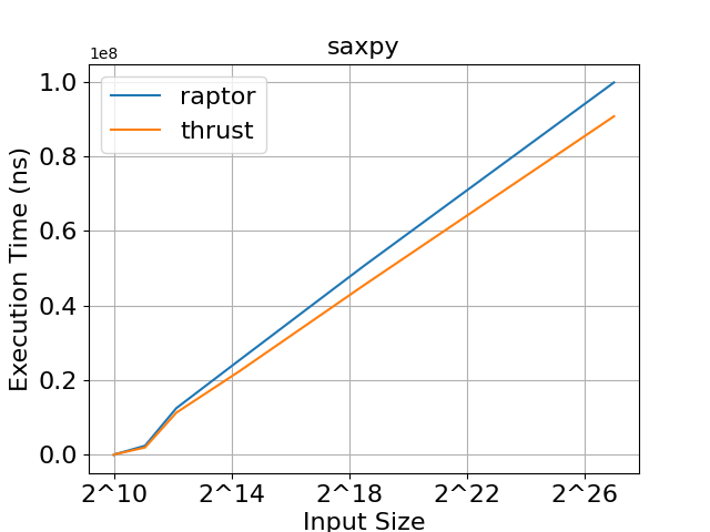
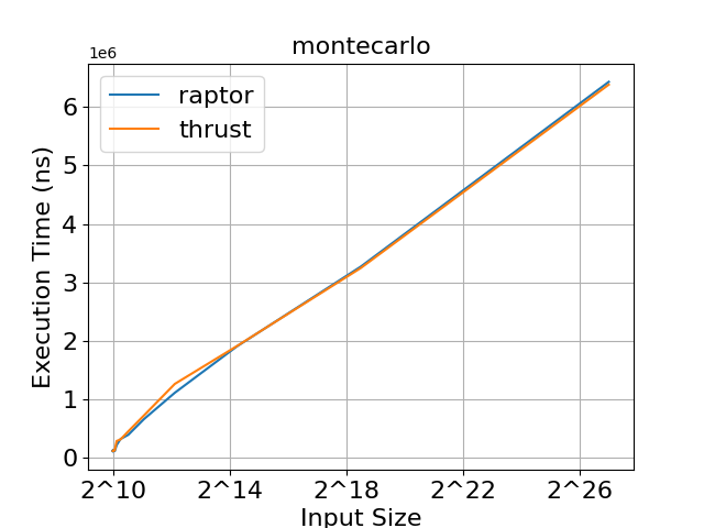
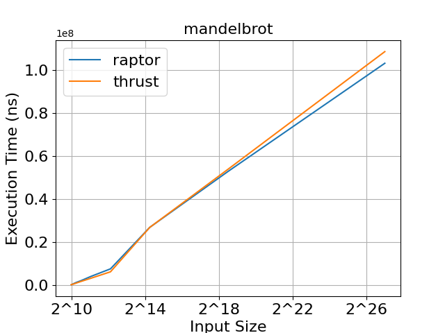
As we can see in figures 2, 3, and 4, raptor and thrust achieve very similar execution times. In saxpy, thrust achieves slightly faster execution times for large input sizes. In montecarlo, both libraries demonstrate practically identical execution times. In mandelbrot, raptor achieves slightly faster execution times for large input sizes. We can conclude that raptor's abstraction doesn't result in any noticeable overheads compared to thrust, and allows for the development of highly efficient programs.
9. Conclusions
Raptor aims to ease the development of efficient parallel applications such that the programmer can focus on the problem related logic rather than constantly dealing with all of CUDA's intricacies. We saw that raptor abstracts all of the host-device communication and allows us to express all computations using skeletons, smart containers and raptor functions. The result is an interface that is both very expressive and more abstract than thrust. Regarding performance, raptor offers almost identical performance to thrust, allowing for extremely efficient programs.
Given that raptor abstracts all CUDA related code, in the future, we would like to offer support for both Nvidia and AMD graphics cards. This can be achieved by isolating the device related code in a CUDA backend module, and replicating this module using HIP. This shouldn't pose much difficulty given HIP's similar syntax to CUDA.